When Most Methods Look Robust: Rethinking GNN Benchmarks for Missing Node Features
TL;DR. Almost every paper on Graph Neural Networks (GNNs) with missing node features uses CORA, CITESEER, and PUBMED as benchmarks, and almost every method looks robust on them. We show this is mostly an artifact of those datasets — their bag-of-words features are already so sparse that adding more missingness barely changes the information available to the model. On dense, semantically meaningful graphs (synthetic, AIR, ELECTRIC, TADPOLE), and under realistic missingness mechanisms (MNAR, distribution shifts), most methods fall apart. A simple baseline that just tells the GNN which entries are missing — we call it GNNmim — holds up across the board.
Full paper: Rethinking GNNs and Missing Features: Challenges, Evaluation and a Robust Solution (Ferrini et al., 2026).
This is a research note on our recent paper. The goal is not to repeat the paper — go read it for the proofs and full experimental tables — but to walk through why we wrote it, what was wrong with the existing evaluation, and what we propose instead.
The setup: GNNs and missing node features
In many real applications of graph neural networks, node features are incomplete. Sensors fail. Patients skip questions. Devices lose connectivity. Formally, given an attributed graph \(G = (V, E, X, Y)\) with feature matrix \(X \in \mathbb{R}^{n \times d}\), we observe only a partial \(X_{\text{obs}}\) together with a missingness mask \(M \in \{0,1\}^{n \times d}\), where \(M_{ij} = 1\) marks an unobserved entry. The task is still node classification, but now the model must learn \(P(Y \mid X_{\text{obs}}, M)\) instead of the clean \(P(Y \mid X)\).
The literature has produced a flurry of architectures for this problem — confidence-guided imputation (PCFI), feature propagation (FP), attention-based attribute completion (FairAC), label propagation hybrids (GOODIE), Gaussian-mixture models (GCNmf), graph-induced sum-product networks (GSPN), and so on. Almost all of them are evaluated the same way: take CORA / CITESEER / PUBMED, drop entries uniformly at random, see how F1 holds up.
That evaluation is broken. Two things are wrong with it.
Problem 1 — the benchmarks are too sparse to expose missingness
CORA, CITESEER and PUBMED use bag-of-words features. Each feature vector is a binary indicator of which words from a vocabulary appear in the paper. The result is feature matrices that are already between 90% and 99% zeros. When most entries are zero anyway, masking some of them out conveys very little new information to the model.
We make this precise. In the paper we prove an information-theoretic bound: under uniform MCAR missingness with rate \(\mu\), the change in mutual information \(\Delta = I(Y; \tilde X) - I(Y; X)\) between labels and features satisfies
\[- n d \, \mu \, h_2\bigl(\mathbb{E}[s(X)]\bigr) \le \Delta \le 0,\]where \(s(X)\) is the feature sparsity and \(h_2\) is the binary entropy. The bound is tight: when sparsity is near 1, the lower bound is tiny, which means no method can lose much information until missingness is extreme — typically above 90%. Empirically you see exactly this: every method stays flat across \(\mu\) on CORA/CITESEER/PUBMED and only collapses near \(\mu = 1\).
So the benchmarks are giving us a flat horizon line and we are mistaking it for robustness.
A second-rate fix: bring in dense, low-dimensional, real-feature graphs
We assemble four datasets that violate the sparsity assumption:
- SYNTHETIC — a Barabási–Albert graph with 5 Gaussian features per node, labels generated by a fixed two-layer GCN on the complete features. Ground truth is known; sparsity is exactly 0.
- AIR — sensor stations measuring CO, NO₂, PM10, O₃, SO₂, plus meteorology. Edges by geographic proximity. Predict PM2.5 category.
- ELECTRIC — buses in the Texas synthetic grid with voltage, angle, and centrality measurements. Predict the operational voltage class.
- TADPOLE — patients in the Alzheimer’s TADPOLE challenge, with clinical scores, CSF biomarkers, and MRI/PET features. Predict diagnostic class.
These all satisfy the RINGS framework properties for benchmark suitability: features and structure are separately informative, and they are complementary rather than redundant.
What that looks like in practice
This is the core diagnostic plot from the paper. Top row: the standard sparse benchmarks. Bottom row: the four dense-feature datasets we propose. Each panel sweeps the missingness rate \(\mu\) from 0 to 1 under structural-MCAR.
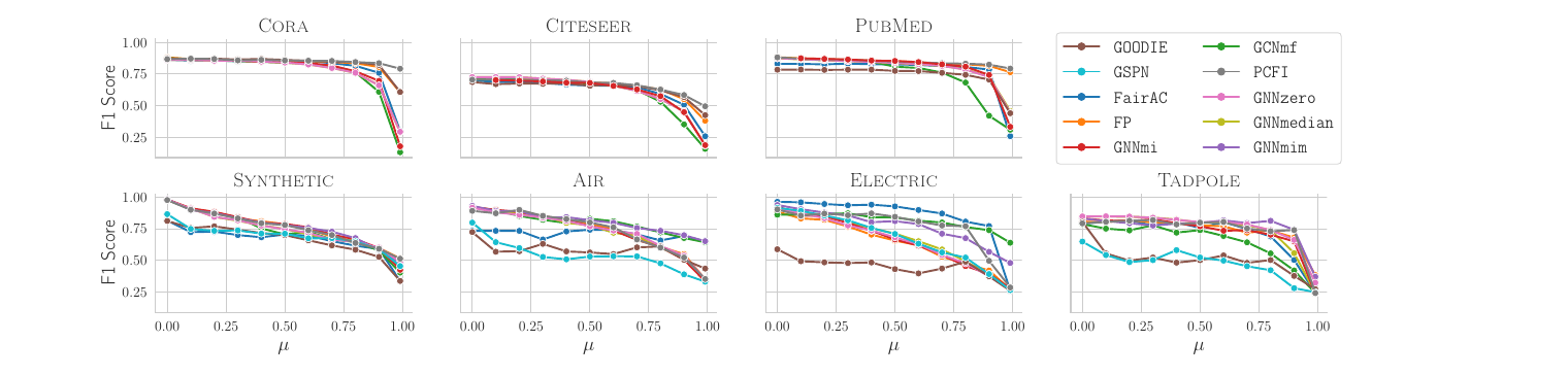
The takeaway: the bottom row is what a useful benchmark looks like. Methods separate, weaknesses become visible, ranking conclusions actually mean something.
Problem 2 — uniform random masking is not how data goes missing in the real world
New to MCAR / MAR / MNAR? I wrote a self-contained primer with Python examples and real-world scenarios from IoT, surveys, and healthcare: MCAR, MAR, and MNAR: A Practical Guide. The rest of this section assumes the basics.
The default missingness mechanism in the literature is U-MCAR: mask each entry independently with probability \(\mu\). A few papers also use S-MCAR, which masks entire feature vectors of randomly chosen nodes. Both are Missing Completely At Random (MCAR) — the missingness is independent of the values and the labels.
Real missingness is rarely MCAR.
- A patient is less likely to disclose their weight when it is unusually high.
- A wearable sensor drops readings during high-motion segments — exactly when the signal is most distinctive.
- A hospital stops collecting a biomarker once a diagnosis is made — leaking the label into the missingness pattern.
These are MNAR (Missing Not At Random) regimes, and they break the implicit assumption behind every imputation-based method that the missingness is ignorable. We design three richer mechanisms that capture this:
- LD-MCAR (Label-Dependent MCAR) — features more informative for the label have a higher probability of being missing, but the per-entry decision is still independent of values.
- FD-MNAR (Feature-Dependent MNAR) — extreme feature values (e.g. high quantiles) are more likely to be missing.
- CD-MNAR (Class-Dependent MNAR) — features that, via a decision tree, predict a particular class are more likely to be omitted for nodes in that class. The intuition: the feature most associated with a diagnosis is the one a patient is most likely to under-report.
We also separate two evaluation regimes:
- R1: same missingness mechanism in train and test (i.i.d.).
- R2: a distribution shift in the missingness — for example, training on FD-MNAR data and testing on U-MCAR. This captures the realistic case where historical training data come from one collection process and deployment data come from another.
Once you sweep the AUC of F1 against \(\mu\) across all five mechanisms and all four datasets, the picture changes a lot:

Different methods are good at different mechanisms. There is no consistent winner among the existing methods — and crucially, the rankings under U-MCAR (the standard evaluation) say very little about the rankings under MNAR.
A simple baseline that holds up: GNNmim
If imputation-based methods rely on assumptions that break under realistic missingness, what is the alternative? A classical idea from the tabular literature: the Missing Indicator Method (MIM). Don’t try to guess the missing values. Instead, tell the model which entries are missing and let it figure out what to do with them.
The graph version is almost embarrassingly simple. We call it GNNmim:
- Replace missing entries with zero (
zero-fill). The zero is just a placeholder; the model is not asked to interpret it as a value. - Concatenate the missingness mask \(M\) as additional binary features.
- Feed the concatenation into a standard GNN (GCN, GraphSAGE, GIN — your choice).
That’s it. No imputation, no MAR assumption, no special training procedure.

The reason this works is structural. Under feature-MAR and label-MAR, the integral over the missing values reduces to the standard classification objective and methods that explicitly model the mask have no theoretical advantage. But under MNAR and under train–test distribution shift in the missingness, the mask carries real predictive signal that imputation cannot recover. By concatenating \(M\) we let the GNN exploit that signal directly.
Distribution shifts: where most methods stumble
The harshest test is regime R2 — train on FD-MNAR with \(\mu_{\text{tr}} = 50\%\), test on U-MCAR with \(\mu_{\text{te}} \in \{0, 25, 50\}\%\). Note that the test missingness is milder, so a method that simply learned to handle missingness rather than memorize a specific pattern should improve.
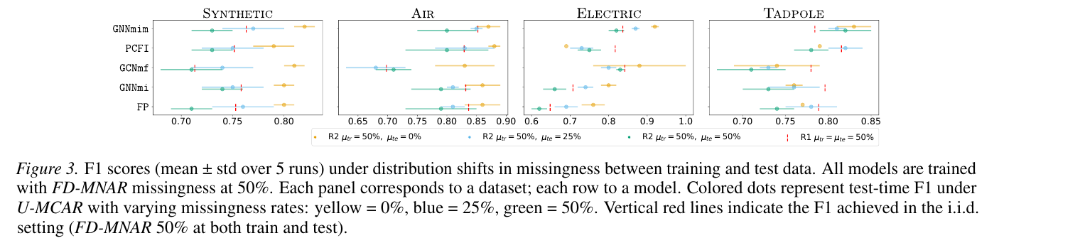
GNNmim sits to the right across all four datasets and all three test rates. It is not always the strict winner under any single condition, but it is never the loser, which is the property you want from a baseline that you intend to deploy.
What this means for the field
Two takeaways, one methodological and one technical:
Methodological. Benchmarks are not just engineering choices — they shape which methods we believe in. The robustness narrative for GNNs with missing features came almost entirely from sparse bag-of-words datasets where any method looks robust. On dense-feature graphs and realistic missingness regimes, most existing methods are not as robust as the literature suggests, and rankings under U-MCAR are not predictive of rankings under MNAR.
Technical. A simple, assumption-free missing-indicator baseline (GNNmim) is competitive with much more elaborate architectures across datasets, mechanisms, and distribution shifts. This is consistent with what the missing-data literature has known for a while — that on tabular data the missing-indicator method is hard to beat — but it had not been studied in the graph setting. The takeaway is not “imputation methods are bad”, but that once you fix the evaluation, simple methods become competitive again and any new architecture should be benchmarked against this baseline.
How to use this if you work in the area
If you are evaluating a new method for GNNs with missing node features:
- Don’t rely on Cora/Citeseer/PubMed alone. Add at least one dense-feature dataset.
- Don’t rely on U-MCAR alone. Test under at least one MNAR mechanism.
- Test under a distribution shift in the missingness. R2-style train/test mismatches are where models that overfit the missingness pattern reveal themselves.
- Compare against GNNmim. If your method does not beat zero-fill + mask concatenation, the gain probably comes from somewhere other than handling missingness well.
The code, datasets and full evaluation harness are in the supplementary material of the paper.
References and further reading
- The full paper: Rethinking GNNs and Missing Features: Challenges, Evaluation and a Robust Solution. arXiv:2601.04855.
- Related work in our group on graph robustness and feature handling is on the publications page.
- A self-contained primer on the three regimes: MCAR, MAR, and MNAR — Practical Guide with Python.
- The Missing Indicator Method on tabular data: Van Ness et al., The Missing Indicator Method: From Low to High Dimensions, KDD 2023.
- On benchmark suitability for graph learning: Coupette et al., No Metric to Rule Them All (2025), and Bechler-Speicher et al., Position: Graph Learning Will Lose Relevance Due to Poor Benchmarks, ICML 2025.
If you have questions or want to discuss the work, my contact is on the about page.