MCAR, MAR, and MNAR: A Practical Guide to Missing Data Mechanisms (with Python)
TL;DR. Statisticians classify missing data into three regimes: MCAR (missing completely at random), MAR (missing at random conditional on observed variables), and MNAR (missing not at random). The distinction is not academic — it determines whether your favorite imputation method is unbiased or silently broken. This post walks through all three with runnable Python examples and real-world scenarios: IoT sensors for MCAR, demographic surveys for MAR, clinical data for MNAR. If you work with incomplete data of any kind, the 10 minutes you spend here will pay off many times over.
The setup
Let \(X\) be a random variable you want to study, and let \(M\) be the missingness indicator: \(M = 1\) if the value is missing, \(M = 0\) if observed. Sometimes you have other observed variables too — call them \(Y\) (these can be features, labels, anything). Following Rubin (1976), the three regimes differ in what \(M\) depends on:
\[\begin{aligned} \text{MCAR:} \quad & P(M \mid X, Y) = P(M) \\ \text{MAR:} \quad & P(M \mid X, Y) = P(M \mid Y) \\ \text{MNAR:} \quad & P(M \mid X, Y) \text{ depends on } X \text{ itself} \end{aligned}\]In words:
- MCAR — the missingness is independent of everything. Pure dice rolls.
- MAR — the missingness depends only on observed variables. Once you know those, the missingness is random.
- MNAR — the missingness depends on the unobserved value itself. You can’t escape it by conditioning on what you see.
This sounds abstract. Let’s make it concrete with three simulations you can copy and run.
MCAR — IoT temperature sensors
A network of temperature sensors reports readings every minute. Sometimes a packet is lost in transit because of network congestion. The packet loss is independent of the temperature value, of the location of the sensor, of the time of day — it is just network noise.
import numpy as np
np.random.seed(42)

# 1000 true temperature readings, normally distributed around 22 °C
n = 1000
true_temp = np.random.normal(loc=22.0, scale=3.0, size=n)

# 30% of readings lost to random network packet drops — MCAR
mcar_mask = np.random.rand(n) < 0.30
observed = true_temp[~mcar_mask]

print(f"True mean:     {true_temp.mean():.2f} °C   (n = {n})")
print(f"Observed mean: {observed.mean():.2f} °C   (n = {len(observed)})")
print(f"Bias:          {observed.mean() - true_temp.mean():+.3f} °C")
True mean:     22.06 °C   (n = 1000)
Observed mean: 22.10 °C   (n = 704)
Bias:          +0.038 °C
The bias is essentially zero. With more samples it would converge to exactly zero. Plotting the two distributions confirms they have the same shape — one is just smaller:
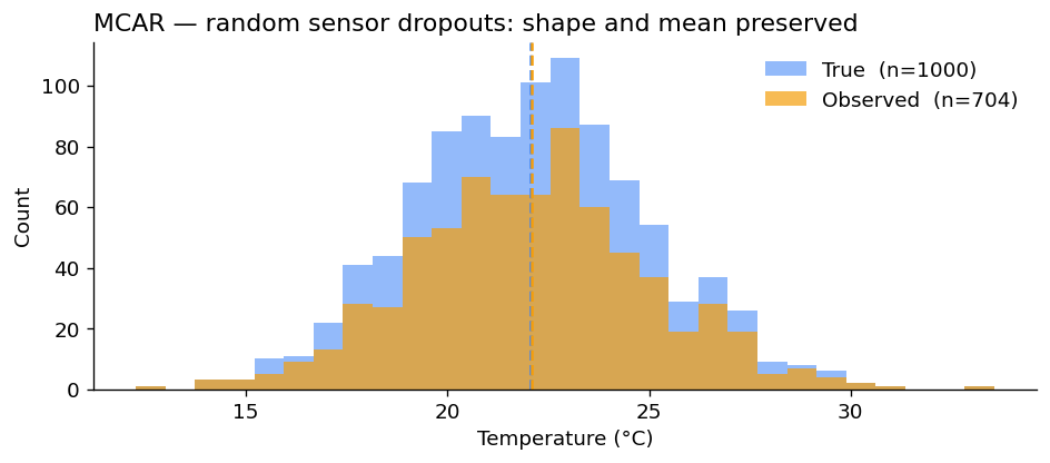
Why this is the easy case. With MCAR, the observed sample is a uniform random subsample of the full data. Any unbiased estimator on the full data is still unbiased on the observed data. Mean imputation, listwise deletion, anything works — at the cost of statistical power, but not of bias.
The catch: MCAR is rare in practice. Truly random missingness occurs in clean engineering settings (packet loss, machine downtime, randomized survey skip patterns), but most real-world missingness has structure.
MAR — Demographic surveys, missingness depends on age
A national income survey asks respondents about their salary. Older respondents are more likely to skip the question — out of privacy concerns, distrust of the surveyor, or simply because the question feels intrusive at certain life stages. Crucially, given a respondent’s age, the actual income value does not affect whether they answer.
This is MAR: missingness depends on age, an observed variable, not on income itself.
np.random.seed(42)
n = 1000
age = np.random.uniform(20, 75, size=n)
# Income increases roughly linearly with age in this synthetic population
income = 15000 + 1500*age + np.random.normal(0, 5000, n)
income = np.clip(income, 12000, 200000)

# Probability of skipping grows with age, from 5% at 20 to 85% at 75.
# Critically, this depends ONLY on age — not on the income value.
p_miss = np.clip((age - 20) / 55 * 0.8, 0.05, 0.85)
mar_mask = np.random.rand(n) < p_miss
observed_income = income[~mar_mask]

print(f"True mean income:         ${income.mean():>9,.0f}")
print(f"Marginal observed mean:   ${observed_income.mean():>9,.0f}")
print(f"Marginal bias:            ${observed_income.mean() - income.mean():>+9,.0f}")
True mean income:         $   85,832
Marginal observed mean:   $   77,077
Marginal bias:            $   -8,756
The marginal observed mean is biased downward by almost $9,000 — because we are losing the high-earning seniors. So far this looks like trouble.
But here’s the key MAR property: conditional on age, there is no bias. Within each age bin the observed mean equals the true mean.
print(f"{'Age bin':<10}{'True':>14}{'Observed':>14}{'Bias':>12}")
for lo, hi in [(20, 35), (35, 50), (50, 65), (65, 75)]:
    in_bin = (age >= lo) & (age < hi)
    t = income[in_bin].mean()
    o = income[in_bin & ~mar_mask].mean()
    print(f"{lo}-{hi:<6} {t:>13,.0f} {o:>13,.0f} {o-t:>+11,.0f}")
Age bin             True      Observed        Bias
20-35            56,190        55,852        -338
35-50            78,418        77,843        -575
50-65           101,389       100,680        -708
65-75           119,910       118,926        -984
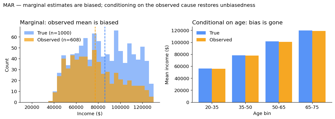
Why MAR is “ignorable”. If you build a model that conditions on age — even a simple regression or a stratified estimator — you recover unbiased estimates of income. Most modern imputation methods (multiple imputation, MICE, regression imputation) assume MAR. They will be correct as long as the missingness depends only on observed variables.
The hard part in practice is believing the data are MAR. You can never fully verify it without seeing the missing values.
MNAR — Patient self-reported weight
Now the textbook hard case. In clinical surveys, patients are asked to self-report their weight. Patients with higher weights are systematically more likely to skip the question. The probability of being missing depends on the value of the weight itself — which is exactly the unobserved quantity you wanted.
np.random.seed(42)
n = 1000
true_weight = np.clip(np.random.normal(78, 14, n), 45, 180)

# Logistic mechanism: heavier patients increasingly likely to skip
p_miss = 1 / (1 + np.exp(-(true_weight - 85) / 8))
mnar_mask = np.random.rand(n) < p_miss
observed_weight = true_weight[~mnar_mask]

print(f"True mean weight:     {true_weight.mean():>5.1f} kg   (n = {n})")
print(f"Observed mean weight: {observed_weight.mean():>5.1f} kg   (n = {len(observed_weight)})")
print(f"Bias:                 {observed_weight.mean() - true_weight.mean():>+5.1f} kg")
True mean weight:      77.8 kg   (n = 1000)
Observed mean weight:  72.2 kg   (n = 635)
Bias:                  -5.6 kg
A 5.6 kg downward bias — clinically meaningful and structural. There is no observed variable you can condition on to make this go away, because the cause of the missingness is the missing value itself.
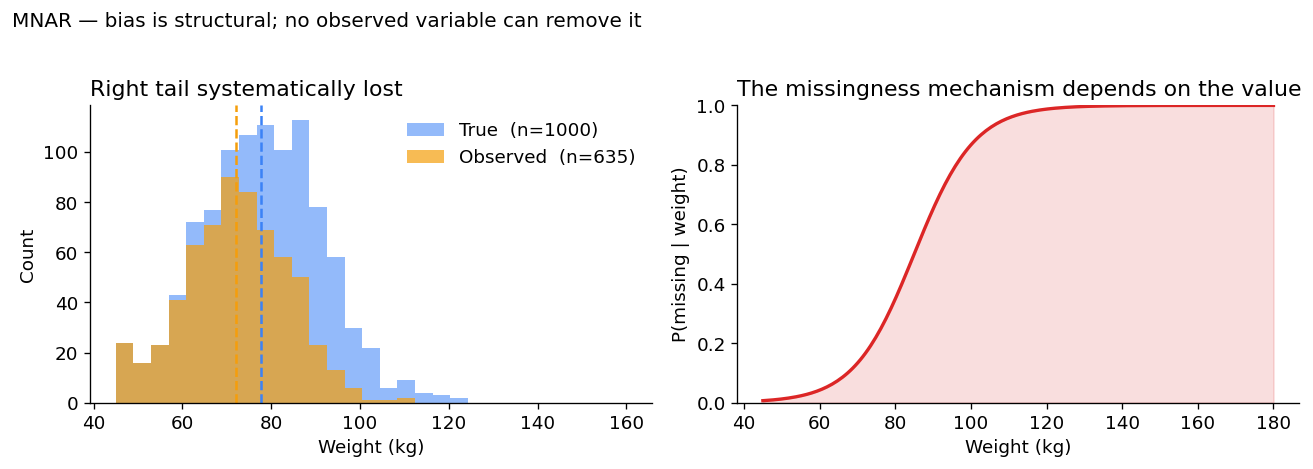
Why MNAR is the dangerous case. Standard imputation methods (mean, MICE, regression on observed variables) are all biased under MNAR — sometimes catastrophically. Recovering correct estimates requires either explicit modeling of the missingness mechanism (which is hard and rarely identifiable) or methods that are assumption-free with respect to the mechanism, like the missing-indicator method which feeds the missingness pattern itself into the model as an extra feature.
Why the distinction matters in practice
Pick any method that handles missing data. It makes one of three assumptions, often implicitly:
| Method | Assumes | Bias under wrong assumption |
|---|---|---|
| Listwise deletion (drop incomplete rows) | MCAR | Biased under MAR and MNAR |
| Mean / median imputation | MCAR | Biased under MAR and MNAR |
| Regression / MICE / multiple imputation | MAR | Biased under MNAR |
| Missing-indicator method | None | Robust across regimes |
| Selection models (Heckman) | MNAR (with strong parametric assumptions) | Biased if mechanism mis-specified |
The most common mistake in applied work is to use a MAR method on MNAR data — because MAR is the default assumption of most software libraries, and most real missingness is at least mildly MNAR.
How to spot which one you have
You cannot test MAR vs MNAR from the data alone — that would require knowing the missing values. What you can do:
- Test MCAR vs not-MCAR. Tools like Little’s MCAR test compare the distributions of observed variables across rows with and without missingness. If they differ, you are not MCAR.
- Reason from the data-generating process. Ask: what causes the missingness? If the answer involves the missing value itself, you have MNAR. If it involves only observed variables, you may have MAR. If it is genuinely independent of everything, MCAR.
- Run sensitivity analyses. Assume different MNAR mechanisms, see how much your conclusions move. If they are stable across plausible MNAR assumptions, you can publish with more confidence.
When this comes up in machine learning
If you train models on data with missing entries — common in healthcare, IoT, recommender systems, finance — the missingness mechanism shapes which methods are valid. A few practical rules:
-
Forget about MCAR. It almost never holds outside controlled experiments. Methods that assume it (
SimpleImputer(strategy="mean"), listwise deletion) are silently biased on real datasets. -
Default to MAR-aware methods.
IterativeImputer, MICE, and any multiple-imputation library assume MAR. They are the right starting point. - Be ready for MNAR. When the missingness pattern itself is informative — e.g. a patient not reporting a symptom is meaningful — feed the mask to the model as an explicit feature. This is the missing-indicator approach, and it generalizes naturally to deep learning, including graph neural networks.
For graph-structured data specifically, I recently wrote a research note on GNNs with missing node features that explores exactly this trade-off — sparse benchmarks make MAR methods look great until you put them under realistic MNAR mechanisms.
References and further reading
- Rubin, D. B. (1976). Inference and Missing Data. Biometrika, 63(3): 581–592. link — the original taxonomy.
- Little, R. J. A., & Rubin, D. B. (2019). Statistical Analysis with Missing Data (3rd ed.). Wiley. The standard textbook reference.
- Van Buuren, S. (2018). Flexible Imputation of Missing Data (2nd ed.). Free online. Excellent, practical, R-flavored but the concepts transfer.
- My research note on GNNs with missing features: Rethinking GNN Benchmarks for Missing Node Features.
Questions or corrections welcome — see the about page for contact.